Tracking in Practice: Student Guide

The tracking framework is you will use for this laboratory hides many of the hairy details behind video decoding and encoding, as well as threading of state through the entire tracking pipeline. It is designed to work under both Linux and Windows. To get the tracking framework, download the zipfile here. Now create a working directory somewhere where you will put all of your work for the practicum. Depending on what operating system you are using, follow these instructions:

You can now test the tracking framework by running:

play_video('car-1.avi');

And to run the basic Kalman filter tracker try this:

kalman_tracker('car-2.avi', 0.05, 50, 3);
kalman_tracker('car-1.avi', 0.05, 50, 3);

Pressing any key while the tracker is running will pause the tracker until you press another key. If anything goes wrong with the framework installation, please contact the practicum instructor.

We have prepared a selection of video sequences for use during the practicum. The videos can be downloaded individually here. You should study these videos carefully, noting the different characteristics of each, the nature of object motion in them and the types of interactions between moving objects. You should also try running the basic tracker provided with the practicum framework on some of these videos.

A tracker in the practicum software framework consists of:

• A segmenter that segments foreground objects from the background;
• a recognizer that identifies which foreground objects are being (or should be) tracked;
• a representer that represents each tracked object in terms of some abstract feature space;
• a tracker that actually does the tracking (i.e. estimates the position of each tracked target in the current frame); and
• an optional visualizer that displays a visualization of each frame of the tracker.

A tracker in the framework requires a Matlab function implementing each of these modules in order to be complete. A tracker (i.e. a collection of processing modules) is modeled in Matlab as structure containing references to each module (that is the Matlab function implementing the module). This structure also contains all state variables that must be passed down the pipeline to other modules. The structure T must contain the following substructures:

1. T.segmenter which must contain a function reference T.segmenter.segment to a function taking the structure T and the current frame.
2. T.recognizer which must contain a function reference T.recognizer.recognize to a function taking the structure T and the current frame.
3. T.representer which must contain a function reference T.representer.represent to a function taking the structure T and the current frame.
4. T.tracker which must contain a function reference T.tracker.track to a function taking the structure T and the current frame.
5. And optionally T.visualizer which must contain a function reference T.visualizer.visualize to a function taking the structure T and the current frame.

We will see a complete example at the end of this section, but once this structure has been created, you can run the tracker on a video using the run_tracker function:

run_tracker(fname, T);

where T is the structure setup previously with references to all of the tracking modules and fname is the filename of the video to run the tracker on. In practice, you will write a wrapper function around run_tracker that sets up the processing pipeline and sets any needed parameters (see the kalman_tracker example at the end of this section).

The segmenter provided performs simple background subtraction based on a rolling-average background model and temporal differencing. The background model is updated like this:

where is a learning rate parameter that controls how quickly the background model incorporates new information and how quickly it forgets older observations. Every pixel in every frame is classified as either background (0) or foreground (1) using a simple threshold:

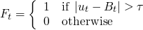
where is a threshold on the difference between a pixel in the current frame and background model. This threshold controls which pixels are classified as foreground. Finally, the foreground image is cleaned a little to close small gaps:

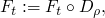
where is the morphological closing operation and is a disk of radius .

The Matlab implementation of this segmenter looks like this (file background_subtractor.m in the framework directory):

function T = background_subtractor(T, frame)

% Do everything in grayscale.
frame_grey = double(rgb2gray(frame));

% Check to see if we're initialized
if ~isfield(T.segmenter, 'background');
  T.segmenter.background = frame_grey
end

% Pull local state out.
gamma  = T.segmenter.gamma;
tau    = T.segmenter.tau;
radius = T.segmenter.radius;

% Rolling average update.
T.segmenter.background = gamma * frame_grey + (1 - gamma) * ...
    T.segmenter.background;

% And threshold to get the foreground.
T.segmenter.segmented = abs(T.segmenter.background - frame_grey) > tau;
T.segmenter.segmented = imclose(T.segmenter.segmented, strel('disk', radius));

return

This is an example of how all modules within the framework work. Each module is passed the global structure T containing all needed parameters (see how the gamma, tau and radius parameters are fished out of the sub-structure segmenter contained in the passed structure T?) and the current frame being processed. The module then does it's processing and stores the results back in the T.segmenter substructure (in the T.segmenter.segmented variable).

Please note that each module is responsible for maintaining its own state parameters and putting them in the structure T. This is the only mechanism by which state is passed to other processing modules and from one frame to the next. Keeping all state variables related to a module local to a substructure (T.segmenter in this case) is good programming practice, and you should do this in all modules that you implement.

The next stage in the pipeline is the recognizer. The basic recognizer provided with the tracking framework is based on simple blob detection. Connected components are found in the segmented image, and the whole set of components is retained as the "recognized" object to be tracked.

The Matlab code for this is simply:

function T = find_blob(T, frame)
T.recognizer.blobs = bwlabel(T.segmenter.segmented);
return

You can see here how the recognizer assumes the segmented image from the previous stage is passed in the T.segmenter.segmented variable. This is an example of how state is passed between processing modules. The recognizer then puts its result in the variable T.recognizer.blob for subsequent modules to use.

It is important to note that the framework does not enforce any particular protocol for passing state variables from module to module. You are responsible for establishing how each module receives its parameters and how it stores its results.

The next module is the representer, which takes the results of recognition and computes a representation of each recognized object to be tracked. In the basic tracker, the representer extracts the BoundingBox and size of each blob and only keeps the biggest one as the single object being tracked. The Matlab code (file filter_blobs.m in the framework directory):

function T = filter_blobs(T, frame)

% Make sure at lease one blob was recognized
if sum(sum(T.recognizer.blobs))
  % Extract the BoundingBox and Area of all blobs
  R = regionprops(T.recognizer.blobs, 'BoundingBox', 'Area');
  
  % And only keep the biggest one
  [I, IX] = max([R.Area]);
  T.representer.BoundingBox = R(IX(size(IX,2))).BoundingBox;
end
return

In a more realistic tracker, the representer module would be responsible for maintaining a list of objects being tracked and establishing correspondences between recognized objects and those currently being tracked.

A simple Kalman filter tracker has been provided in the practicum framework. It uses the results of the representer to track the position and extent of the object being tracked. The Kalman filter works by estimating an unobservable state which is updated in time with a linear state update and additive Gaussian noise. A measurement is provided at each time step which is assumed to be a linear function of the state plus Gaussian noise. It is the most complex module in the framework, and receives and stores a large amount of state information. Here is the Matlab function (file kalman_step.m in the framework directory):

function T = kalman_step(T, frame)

% Get the current filter state.
K = T.tracker;

% Don't do anything unless we're initialized.
if isfield(K, 'm_k1k1') && isfield(T.representer, 'BoundingBox')

  % Get the current measurement out of the representer.
  z_k = T.representer.BoundingBox';
  
  % Project the state forward m_{k|k-1}.
  m_kk1 = K.F * K.m_k1k1;
  
  % Partial state covariance update.
  P_kk1 = K.Q + K.F * K.P_k1k1 * K.F';
  
  % Innovation is disparity in actual versus predicted measurement.
  innovation = z_k - K.H * m_kk1;
  
  % The new state covariance.
  S_k = K.H * P_kk1 * K.H' + K.R;
  
  % The Kalman gain.
  K_k = P_kk1 * K.H' * inv(S_k);
  
  % The new state prediction.
  m_kk = m_kk1 + K_k * innovation;
  
  % And the new state covariance.
  P_kk = P_kk1 - K_k * K.H * P_kk1;
  
  % Innovation covariance.
  K.innovation = 0.2 * sqrt(innovation' * innovation) + (0.8) ...
      * K.innovation;
  
  % And store the current filter state for next iteration.
  K.m_k1k1 = m_kk;
  K.P_k1k1 = P_kk;
else
  if isfield(T.representer, 'BoundingBox');
    K.m_k1k1 = T.representer.BoundingBox';
    K.P_k1k1 = eye(4);
  end
end

% Make sure we stuff the filter state back in.
T.tracker = K;

return

You should study this function carefully to see how the tracker is initialized and how it maintains its state information.

The final module in the processing pipeline is the visualizer. It is not mandatory, but it is always a good idea to provide a minimal visualizer to see how your tracker is performing. The visualizer provided simply displays the current frame with rectangles indicating the current detection and current estimate (file visualize_kalman.m in the framework directory):

function T = visualize_kalman(T, frame)

% Display the current frame.
imshow(frame);

% Draw the current measurement in red.
if isfield(T.representer, 'BoundingBox')
  rectangle('Position', T.representer.BoundingBox, 'EdgeColor', 'r');
end

% And the current prediction in green
if isfield(T.tracker, 'm_k1k1');
  rectangle('Position', T.tracker.m_k1k1, 'EdgeColor', 'g');
end
drawnow;
return

A more fancy (and useful) visualizer would also display quantitative information about the internal state of the tracker (for example a real time plot of the Kalman innovation term). This is very useful to get a clear picture of what that tracker is actually doing.

Now that we have a Matlab function implementing all of the pieces of the processing pipeline, we can string them together using the run_tracker function in the framework. For the provided modules, the function kalman_tracker does just this:

function T = kalman_tracker(fname, gamma, tau, radius);
% Initialize background model parameters
Segmenter.gamma   = gamma;
Segmenter.tau     = tau;
Segmenter.radius  = radius;
Segmenter.segment = @background_subtractor;

% Recognizer and representer is a simple blob finder.
Recognizer.recognize = @find_blob;
Representer.represent = @filter_blobs;

% The tracker module.
Tracker.H          = eye(4);        % System model
Tracker.Q          = 0.5 * eye(4);  % System noise
Tracker.F          = eye(4);        % Measurement model
Tracker.R          = 5 * eye(4);    % Measurement noise
Tracker.innovation = 0;
Tracker.track      = @kalman_step;

% A custom visualizer for the Kalman state.
Visualizer.visualize = @visualize_kalman;

% Set up the global tracking system.
T.segmenter   = Segmenter;
T.recognizer  = Recognizer;
T.representer = Representer;
T.tracker     = Tracker;
T.visualizer  = Visualizer;

% And run the tracker on the video.
run_tracker(fname, T);
return

This function creates the global tracker structure T, initialized with all of the substructures (segmenter, recognizer, representer, tracker and visualizer). Each of these substructures is initialized with the required function reference and all parameters required. Finally, the run_tracker function executes the processing pipeline on the video passed in as a parameter.

You can run the basic tracker on a video using (for example):

kalman_tracker('car-2.avi', 0.05, 20, 3);

Segmentation (in the context of tracking) is the process of separating the foreground objects from the background of the video sequence. When working on these exercises, always keep in mind what the purpose of the segmenter is in terms of the overall tracking problem.

Detection is the process of identifying which of the segmented foreground objects are of interest to the tracking.

Once an object has been segmented and detected, it and its kinetic properties must be represented in some way. These exercises are designed to illustrate how the choice of representation is key for tracking of visual phenomena.

And finally, tracker. The reason we're all here…

If you have an idea for an exercise that you would like to complete in lieu of one of the mandatory ones, please speak with the practicum instructor to make you proposal. Particularly approciated would be proposals for improving the tracking framework (for example, matlab classes instead of structures).

The practicum exercises will be done in groups of two (2) or three (3) people. There will be no exceptions to this rule. Groups should be formed by November 28th, and one (1) representative from each group should email bagdanov@dsi.unifi.it with your group members. Please use the prefix "DBMM Tracking:" in the subject of your email.

Each group will prepare a final report of at most fifteen (15) pages. This report should contain a qualitative and quantitative critical analysis of the work each group has done on the practicum exercises. It should contain the following sections:

1. Introduction - which introduces the report with an overview of the work done, a brief description of the problems chosen, and insights gained through the exercise.
2. Segmentation - containing a detailed account of the mandatory and optional exercises done on the subject of segmentation.
3. Detection - containing a detailed account of what you did (and learned) regarding the detection problem.
4. Representation - containing a detailed account of how the representation problem was approached.
5. Tracking - containing a detailed account of what you did for the tracking module exercises.
6. Conclusions - a concluding section that discusses the overall tracking system as explored and implemented by the group through the exercises.

In each of the main sections (2-5) you should discuss both the mandatory and optional practicum exercises that you completed. You should discuss the theoretical properties you expected from your implementation, and also the technical details of problems encountered during implementation. Where possible, you should draw links between these sections. For example, if you implemented a representation specifically because of the type of tracker you used, this dependence should be made clear in your report. Section 6 should contain the most important conclusions about your experience with all individual modules as well as overall conclusions about the behavior and performance of the overall tracking system developed.

Technical writing is a difficult skill to master. Some very experienced writers claim that it can never be mastered, but only practiced. You should include graphics and figures where appropriate, source code if necessary to illustrate a point, and above all strive to express your ideas and observations clearly and concisely. Most importantly, you should be careful to qualify the performance of your trackers by stating the assumptions made about what situations it should be applied. Don't be afraid to include negative examples where you tracker fails if it serves to illustrate a point. This is an excellent opportunity to practice and improve your writing abilities.

Please note: all final reports should be accompanied with a zipfile containing all source code for all implemented exercises. This source code should be clearly documented, and should also contain instructions for running developed trackers on standard sequences. The quality of your source code will be a factor in determining your final grade.

VERY IMPORTANT: We encourage collaboration and learning from examples available on the internet. But all source code submitted for the practicum must be the sole work of the practicum group submitting it. Studying the implementation of someone else is always a good idea, but you must synthesize the ideas into your own implementation. If you must include code from someone else, make sure you include the correct attribution of ownership in the source code and in your report. Code copied and pasted from the internet or from other students without attribution is plagiarism and your grade will suffer.

The final grade for the tracking lab will be determined on a scale from 0 to 100. The grade will be computed on the basis of:

Participation	10%
Source code quality	10%
Final report	20%
Mandatory exercises	30%
Optional exercises	30%

The exercises, mandatory and optional, must be discussed in your report and all related source code submitted with the final report.

Remember: you must complete all mandatory exercises and two (2) optional ones (from two different categories) in order to receive full credit for the tracking lab.

The following lectures, discussion sessions and presentations have been scheduled:

Date	Topic
28/11/2011	Tracking lab day 1
02/12/2011	Tracking lab day 2
16/12/2011	Final reports due